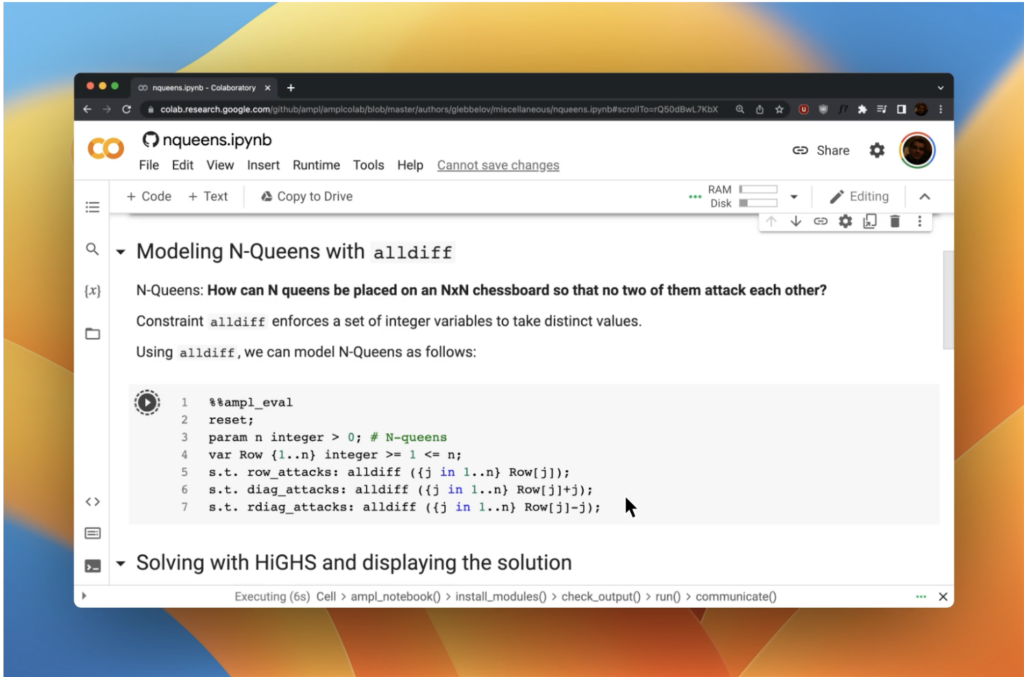
Experience the All-New Python Ecosystem for Large-Scale Optimization
Natural mathematical modeling syntax + natural python integration.
Experience the All-New Python Ecosystem for Large-Scale Optimization
Natural mathematical modeling syntax + natural python integration.
AMPL Model Colaboratory is a collection of AMPL models in Jupyter Notebooks that run on platforms such as Google Colab, Kaggle, Gradient, and AWS SageMaker.
Bring optimization to your courses easily with models on Google Colab, or a free, easily distributed AMPL for Courses license.
Deployment is easy with solvers now available as python packages. Deploy in the cloud using Docker containers, or with options such as cloud functions (e.g. AWS Lambda and Azure Functions)
Performance of heavily optimized C code without losing model readability
The amplpy interface allows developers to access the features of AMPL from within Python. With amplpy you can model and solve large-scale optimization problems in Python leveraging the performance of heavily optimized C code without losing model readability.
In the same way that AMPL’s syntax matches naturally the mathematical description of the model, the input and output data matches naturally Python lists, sets, dictionaries, pandas and numpy objects.
All model generation and solver interaction is handled directly by AMPL, which leads to great stability and speed; the library just acts as an intermediary, and the added overhead (in terms of memory and CPU usage) depends mostly on how much data is sent and read back from AMPL, the size of the expanded model as such is irrelevant.

All AMPL commercial and open-source solvers are available as Python Packages
Now available as Python Packages for Windows, Linux, and macOS. Easy to install in just a few lines of code.
					# Install Python API for AMPL
$ python -m pip install amplpy --upgrade

# Install HiGHS and Gurobi (AMPL is installed automatically with any solver)
$ python -m amplpy.modules install highs gurobi

# Activate your license (e.g., free https://ampl.com/ce license)
$ python -m amplpy.modules activate <license-uuid>

# Confirm that the license is active
$ python -m amplpy.modules run ampl -vvq

# Import in Python
$ python
>>> from amplpy import AMPL
>>> ampl = AMPL() # instantiate AMPL object
Collaborate and model for free on Google Colab
AMPL on Google Colab is enabled with a default Community Edition license to allow freedom to model without limitations on variables or constraints for personal, academic, and commercial prototyping purposes. Model with open-source solvers or activate your own Community Edition license for commercial solver trials.
Load data directly from python data structures using amplpy
Solve with commercial and open-source solvers and retrieve your solution. Switch out solvers in one line of code and solve again for a new solution.

More ways to collaborate
Build and share data apps quickly with Streamlit – no front-end experience necessary.
Not just for Google Colab, our collection of AMPL models in Jypyter Notebooks run in Kaggle, Gradient, and AWS Sagemaker.

Linear Optimization in Python
AMPL stands out in the realm of linear programming within Python due to its intuitive model formulation, seamless integration with Python, and flexibility in solver compatibility. Its design allows users to articulate optimization problems with a syntax that mirrors mathematical expressions, enhancing readability and ease of use. This simplicity is invaluable when combined with Python, known for its straightforward syntax and extensive libraries for data processing and analysis.
The integration between AMPL and Python facilitates a streamlined workflow, where data can be effortlessly manipulated and visualized in Python before and after optimization in AMPL. This interoperability is crucial for embedding linear programming models into broader analytical frameworks, making AMPL a versatile tool in various applications from logistics to energy management.
Finally, AMPL’s ability to interface with multiple high-performance solvers ensures that users can find the most efficient solutions to their problems. This solver flexibility, coupled with Python’s capabilities for automation and extensive data handling, positions AMPL as a powerful and efficient choice for tackling linear programming challenges in a Python-centric environment.
Mixed Integer Optimization in Python
Mixed Integer Programming (MIP) goes beyond traditional linear programming by allowing you to incorporate integer variables, crucial for real-world problems involving whole numbers like machine quantities or on/off decisions.
This text leverages the power of Python and AMPL to make MIP accessible.
We’ll guide you through defining variables, constraints, and objectives intuitively, empowering you to tackle complex optimization challenges in various domains like logistics and production scheduling. Unleash the full potential of MIP in Python to make informed decisions with real-world impact.
Network Optimization in Python
Network optimization in Python, especially for AMPL users, combines Python’s data handling capabilities with AMPL’s optimization modeling power.
Integrating Python with AMPL enables users to dynamically generate and solve optimization models, leveraging Python for data preprocessing and post-processing of results.
Together these frameworks address intricate network optimization challenges, making it an invaluable approach for professionals seeking to optimize transportation, logistics, or data communication networks efficiently.
Convex Optimization in Python
Convex optimization offers powerful tools for solving problems with guaranteed optimal solutions.
This section explores how Python and AMPL empower you to harness the power of convexity. We’ll delve into formulating optimization problems, utilizing Python’s rich ecosystem for data manipulation, and leveraging AMPL’s robust solving capabilities.
Master techniques like linear, least squares, and portfolio optimization to make informed decisions across various disciplines. Join us as we unlock the potential of convex optimization in Python for achieving optimal outcomes in finance, engineering, and beyond.
Conic Optimization in Python
Conic optimization, a class of optimization problems characterized by conic constraints, is pivotal for various applications that require robust and efficient solutions. Python, through AMPL, provides sophisticated tools for formulating and solving conic optimization problems.
AMPL enables users to express problems in a high-level, intuitive manner while ensuring powerful computational techniques under the hood for solving large-scale conic optimizations.
Integrating Python with AMPL, a language designed for high-complexity optimization models, allows for a seamless workflow that combines AMPL’s advanced modeling capabilities with Python’s flexibility in data handling and post-solution analysis.
Stochastic Optimization in Python
Stochastic optimization deals with optimization problems under uncertainty, focusing on finding optimal solutions in environments where randomness in data or models affects decision-making. Integrating AMPL, a powerful modeling language for optimization, with Python’s computational ecosystem, including libraries like NumPy and SciPy, provides a robust framework for tackling stochastic optimization challenges.
Leveraging AMPL for high-level model formulation and Python for data processing and algorithmic implementation offers a comprehensive approach for solving complex stochastic optimization tasks across various domains.
Robust Optimization in Python
Robust optimization is a strategy for dealing with optimization problems under uncertainty, aiming to find solutions that remain effective under various scenarios of data and model parameters.
By integrating AMPL’s sophisticated modeling capabilities with Python’s robust computational libraries, practitioners can address complex robust optimization tasks.
This approach allows for the precise modeling of uncertainties and the development of solutions that are immune to the worst-case scenarios of these uncertainties. Utilizing AMPL for defining optimization models and Python for scenario analysis and data handling creates a powerful synergy.

Python for Portfolio Optimization
Python, with its robust ecosystem like NumPy and pandas, facilitates efficient data manipulation and analysis for financial assets. AMPL, an algebraic modeling language, allows you to formulate optimization models for portfolio construction.
This powerful combination enables the application of advanced techniques like Mean-Variance Optimization and Capital Asset Pricing. By leveraging Python and AMPL, you can construct portfolios that optimize risk-return tradeoff based on historical data and desired risk tolerance, leading to informed investment decisions.
Python for Marketing
Python and AMPL offer valuable tools for marketers and analysts as well. Python’s powerful data manipulation and analysis libraries like pandas and scikit-learn empower marketers to segment customers and optimize campaigns based on insights gleaned from their data.
AMPL allows formulation of optimization models for efficient resource allocation and budget distribution across different marketing channels or customer segments.
Additionally, Python’s machine learning capabilities combined with AMPL’s optimization power can be harnessed to optimize pricing strategies based on predicted demand, leading to data-driven decisions and improved marketing effectiveness. However, this application requires a strong foundation in both Python and AMPL, along with marketing analytics concepts.
Python for Network Engineering
Beyond their traditional uses, Python and AMPL offer a surprising toolkit for network engineers. Python’s libraries like NetworkX empower engineers to model and optimize network designs, while AMPL allows formulating mathematical models for efficient network configuration.
Python’s data analysis capabilities combined with AMPL’s optimization power can be harnessed for tasks like traffic routing, resource allocation, and even network security optimization. However, effectively using this duo requires expertise in both Python and AMPL, alongside a solid foundation in network engineering principles.
AMPL APIs are included in all licenses. Start free today with a Community Edition license to start using amplpy.
AMPL APIs are included in all licenses. Start free today with a Community Edition license to start using amplpy.
Getting started with AMPL is easy – with our documentation, free licenses, AMPL modeling book, and tutorial (coming soon!)